Python for Excel Analysts: Combining Tables

This is the final blog post in a series that teaches you how to work with tables of data using Python code. The subject of this post is a common operation used to prepare data for analysis—combining tables. 

As a Microsoft Excel analyst, you’ve likely used Excel functions like VLOOKUP() and XLOOKUP() to combine data tables.

It’s the same in the world of Python. Combining data tables (i.e., “joins”) is a very common operation. Using Python to join tables of data provides you with three significant advantages in this regard:

• The pandas library offers a complete set of various table join operations commonly used to prepare data for advanced analytics.
• A greater level of control over how tables of data are joined. 
• Standardizing your joining logic so others can quickly reproduce it.

If you’re unfamiliar with the pandas library, check out Part 1 of this blog series.

Each post in the series has an accompanying Microsoft Excel workbook to download and use to build your skills. This post’s workbook is available for download here.

For convenience, here are links to all the blog posts in this series:

• Part 1 – The Basics
• Part 2 – Working with Columns
• Part 3 – Filtering Tables 
• Part 4 – Data Cleaning and Wrangling
• Part 5 – Combining Tables (this post)

Note: To reproduce the examples in this post, install the Python in Excel trial.

Combining Tables in Excel

While not the only way to combine data tables, Excel’s VLOOKUP() function is the most used historically. Other options include XLOOKUP()  and the combination of INDEX() and MATCH() functions.

This blog post will use VLOOKUP() to explore the relevant concepts for joining data tables and then map these concepts to the features of pandas DataFrames.

The Data Tables

This blog post will use a more realistic example of data tables compared to what was used in the previous blog posts.

First, the InternetSales table:

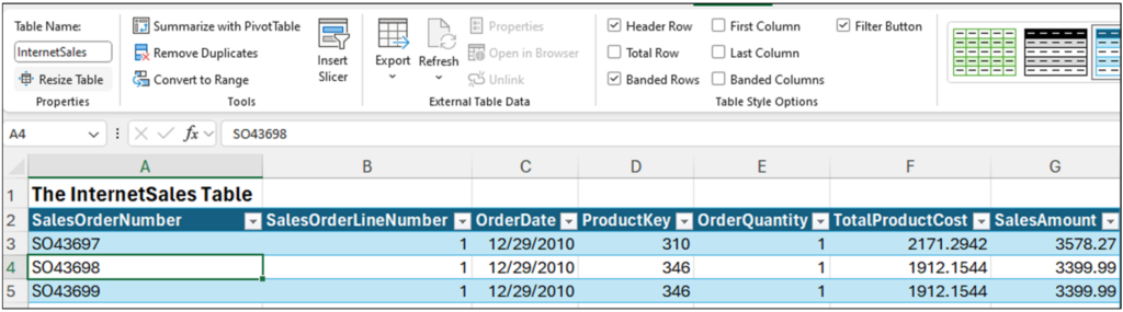
Fig 1 – The InternetSales Excel table

As depicted in Fig 1, the InternetSales table is more representative of data you might see in the real world. For example, if the data was sourced from a data warehouse.

Next up is the ProductInfo table:

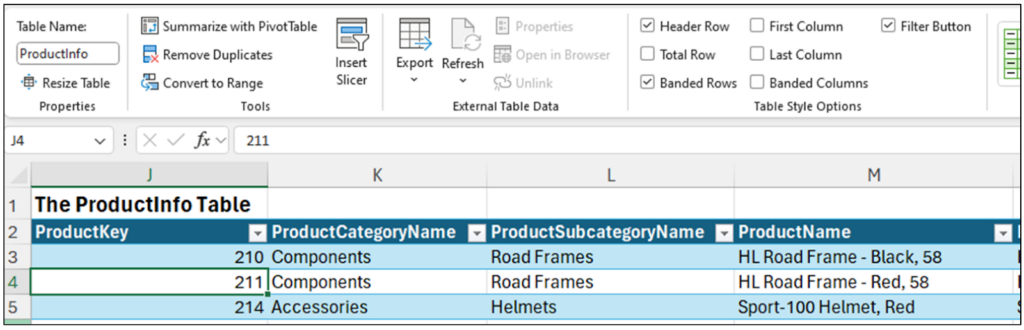
Fig 2 – The ProductInfo Excel table

The two tables represent a classic scenario for joining data – the InternetSales’ ProductKey column allows for looking up the textual descriptions of the products stored in the ProductInfo table.

Traditionally, the VLOOKUP() function has been used for this scenario.

Combining the Tables with VLOOKUP

Let’s say you would like to add a ProductCategoryName column to InternetSales to facilitate a data analysis you would like to perform. The Excel code to make this happen is straightforward:

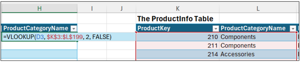
Fig 3 – Excel code to join the tables using VLOOKUP

Hitting the <Enter> key populates the Excel code down the rows of the InternetSales table. Looking at the ProductCategoryName column’s filter dialog shows all the unique values populated in the column from the join:

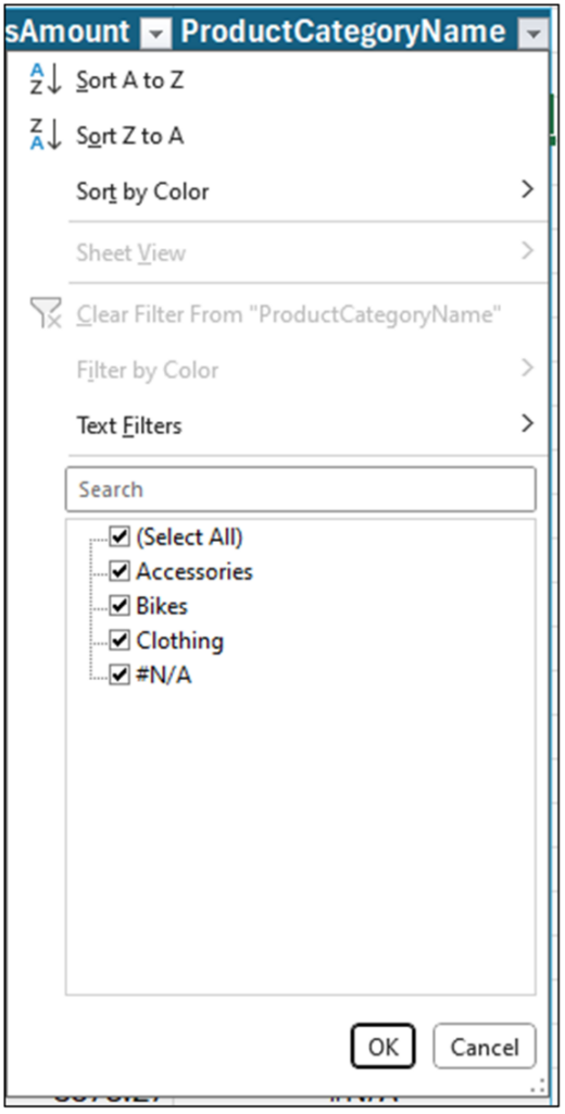
Fig 4 – The filter dialog of the new ProductCategoryName column

While this is a contrived example to be sure, it provides a solid foundation for mapping your Excel knowledge to joining DataFrames using the pandas library.

Mapping Your VLOOKUP Knowledge

The first concept in mapping our knowledge is thinking of two data tables to be joined as being on the “right” side of the join and the “left” side of the join. 

In the example above, InternetSales is the left table, and ProductInfo is the right table: 

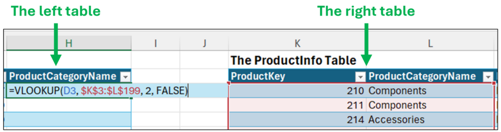
Fig 5 – The left and right tables of the join

The next concept is known as the “join condition.” Using the Excel code depicted in Fig 5, the join condition is where the value of the ProductKey column of the left table (e.g., cell D3) matches the value of the ProductKey column of the right table (i.e., cells $K$3:$K$199).

When the join is run in Excel, notice that not every cell in the new ProductCategoryName column contains a value:

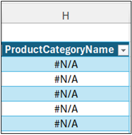
Fig 6 – Missing data in the ProductCategoryName columns

The behavior of the VLOOKUP() function is to return values when the join condition has a match and to return no value (i.e., #N/A) when there is no join condition match. This behavior is called a “left join” in many programming languages (e.g., SQL, Python, R, etc.).

BTW – The absence of value is typically denoted “null” or “NaN” (“not a number”) when using pandas.

Lastly, note how the VLOOKUP() function only joins a single column of data by default. As you will see, this is not the default behavior when joining pandas DataFrames.

Combining Tables in Python

Before exploring how to perform joins, the Excel table data must be loaded into pandas DataFrame objects.

First, use the PY() function to create your Python formula:

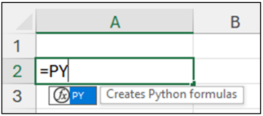
Fig 7 – Call the Excel PY() function

Next, when you type the “(“ the will indicate it contains Python code:

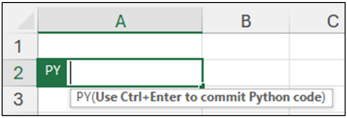
Fig 8 – An Excel Python cell

Here’s the code to load the InternetSales Excel table as a pandas DataFrame:

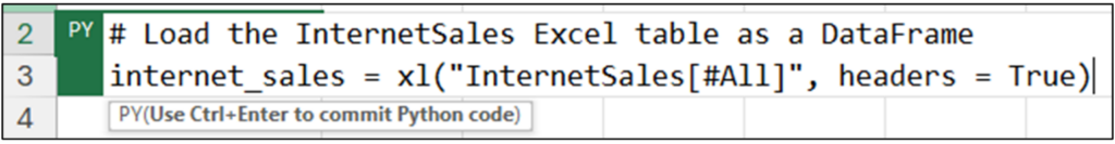
Fig 9 – Constructing a DataFrame from the InternetSales Excel table

Hitting <Ctrl+Enter> on your keyboard will execute the code. Assuming the code was entered correctly, you will see something like the following:

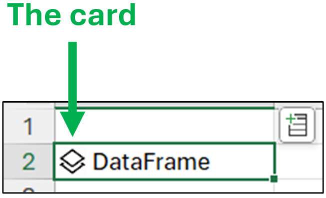
Fig 10 – Successfully loading the InternetSales data as a DataFrame

Clicking the card gives you a preview of the DataFrame object:

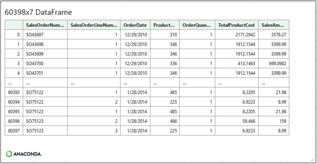
Fig 11 – The card for the internet_sales DataFrame

This process needs to be repeated for the ProductInfo Excel table. Here’s the code:

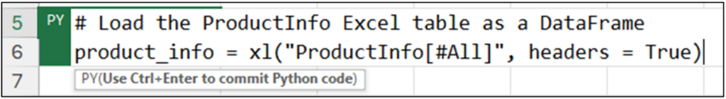
Fig 12 – Constructing a DataFrame from the ProductInfo Excel table

With the DataFrame objects constructed, it’s time to perform some joins.

Left Joins

The pandas DataFrame class has a join() and a merge() method to combine DataFrames. It turns out that the merge() method is conceptually more like Microsoft Excel, so merge() will be used instead of join() for this post.

BTW – If you want to learn more, check the online documentation for merge() and join().

As covered in the previous section, one of the most common way to combine tables is to use a left join (e.g., like VLOOKUP). Conceptually, this is how a left join works using pandas DataFrames:

• Data from the right table will be added to the left table where there is a match.
• Where there is no match, “NaNs” (i.e., “not a number”) will be added to the left table.
• Matching uses a specified join condition.

The following Python code implements the same left join shown in the previous section using VLOOKUP():

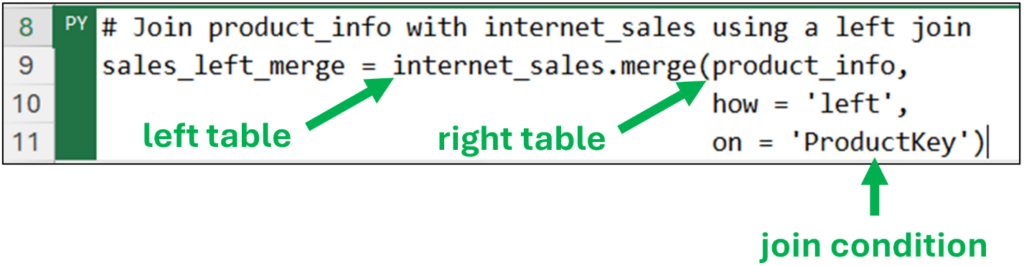
Fig 13 – Using a left join to combine the internet_sales and product_info DataFrames

Note – The code depicted in Fig 13 appears on multiple lines because the cell is set to Wrap Text using the Excel Ribbon.

As depicted in Fig 13, the merge() method returns a new DataFrame object with the combined data. The original DataFrames remain unchanged.

Executing the code and clicking the cell’s card provides a preview of the sales_left_merge DataFrame:

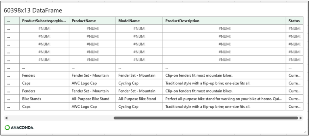
Fig 14 – The card for the sales_left_merge DataFrame

Note – Python “NaN” values are displayed in Excel as #NUM! and denote a missing value.

Compare the results depicted in Fig 14 to those from VLOOKUP() in Fig 3. By default, VLOOKUP() only joins a single column from the right table, while the DataFrame’s merge() method joins all the columns from the right table.

Left joins are very commonly used in data analysis scenarios, but they are not the only commonly used join.

Inner Joins

Another commonly used join in data analysis is the “inner join.” Conceptually, this is how an inner join works using pandas DataFrames:

• Data from the right table will be added to the left table where there is a match.
• Where there is no match, “NaNs” (i.e., “not a number”) will be added to the left table.
• Any rows in the left table containing NaNs for the right table columns are removed.
• Matching uses a specified join condition.

The difference between left and inner joins is how many rows are kept. With left joins, all rows from the left table are kept, while an inner join removes rows with no matches from the left table.

Here’s the code for using an inner join between the internet_sales and product_info DataFrames:

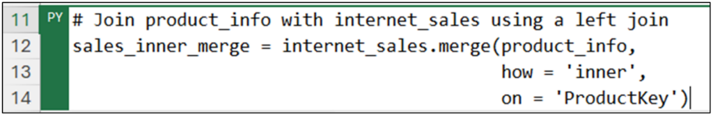
Fig 15 – Using an inner join to combine the internet_sales and product_info DataFrames

Note – The code depicted in Fig 15 appears on multiple lines because the cell is set to Wrap Text using the Excel Ribbon.

After the inner join code runs, clicking on the card provides the following preview of the sales_inner_merge DataFrame:

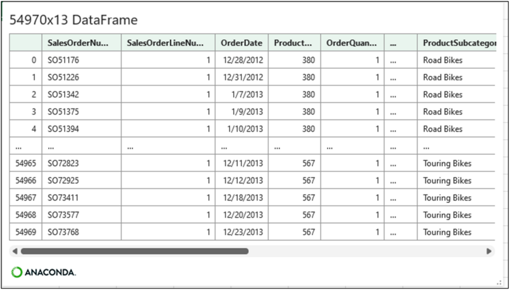
Fig 16 – The card for the sales_inner_merge DataFrame

Compare the cards depicted in Fig 11, Fig 14, and Fig 16. The row counts of Fig 11 and Fig 14 are the same at 60,398. 

By way of comparison, Fig 16 has a row count of 54,970. That means 5,428 rows of the internet_sales DataFrame could not be matched with data in the product_info DataFrame.

While even more types of joins are available using DataFrames, left and inner joins are used most of the time. 

More Join Goodness

This blog post has been an introduction to joining pandas DataFrames. The merge() method provides many more features (e.g., using multiple join conditions) than could be covered in this post. 

If you are interested in learning more, be sure to check out the online documentation.

What’s Next?

This blog series has provided a great foundation for working with data tables using Python, but there is much more to learn. Consider the following a step-by-step guide for what to learn next.

First, there is much more to learn about how to use pandas to prepare your data for analysis. If you liked this blog series, check out my Anaconda-certified course Data Analysis with Python in Excel. 

Second, learning more about data cleaning and wrangling will serve you well. The best analyses come from the best data. To learn more, Anaconda offers the Data Cleaning with pandas course.

Next up is data visualization. Python offers the ability to easily create powerful data visualizations that allow you to glean insights from your data. Data visualization is not only an analysis technique in its own right but also a critical step in conducting advanced analytics. To learn more, be sure to check out Anaconda’s course Introduction to Data Visualization with Python.

Lastly, using Python unlocks a world of advanced analytics. A good place to start your advanced analytics journey is with an Introduction to Machine Learning.

I hope you have found this blog series useful and are excited about the possibilities of running Python code inside of Microsoft Excel.

Until next time, stay healthy and happy data sleuthing!

Disclaimer: The Python integration in Microsoft Excel is in Beta Testing as of the publication of this article. Features and functions are likely to change. Don’t hesitate to reach out if you notice an error on this page. 

Bio

Dave Langer founded Dave on Data, where he delivers training designed for any professional to develop data analysis skills. Over the years, Dave has trained thousands of professionals. Previously, Dave delivered insights that drove business strategy at Schedulicity, Data Science Dojo, and Microsoft.