This is the third in a series of blog posts that explains how to work with tables of data using Python code. The subject of this post is one of the most common operations performed when analyzing data: filtering tables.
The most impactful analyses are born from the best data. Filtering your data using the Python pandas library provides you with two big advantages:
Tremendous power and flexibility to define your filters
Standardizing the filtering process so that it is quickly reproducible by others
Each post in the series has an accompanying Microsoft Excel workbook to download and use to build your skills. This post’s workbook is available for download here.
For convenience, here are links to all the blog posts in this series:
As an Excel analyst, one of the most common operations you perform is filtering a data table to a subset of the data you need for the analysis at hand. Not surprisingly, Microsoft Excel provides you with many options for filtering tables.
Your knowledge of Excel filtering makes learning how to filter data tables using Python straightforward. The key is to map your Excel filtering knowledge to how you accomplish the same results using the pandas library.
This blog post will map three of the most common Excel filtering scenarios to Python code:
Filtering on a single value in a single column
Filtering on multiple values in a single column
Filtering on multiple columns
Single Value Filtering
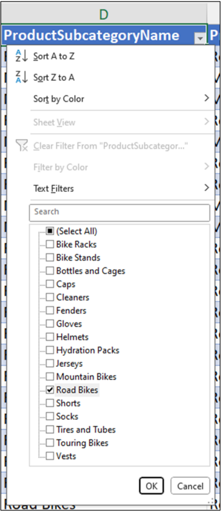
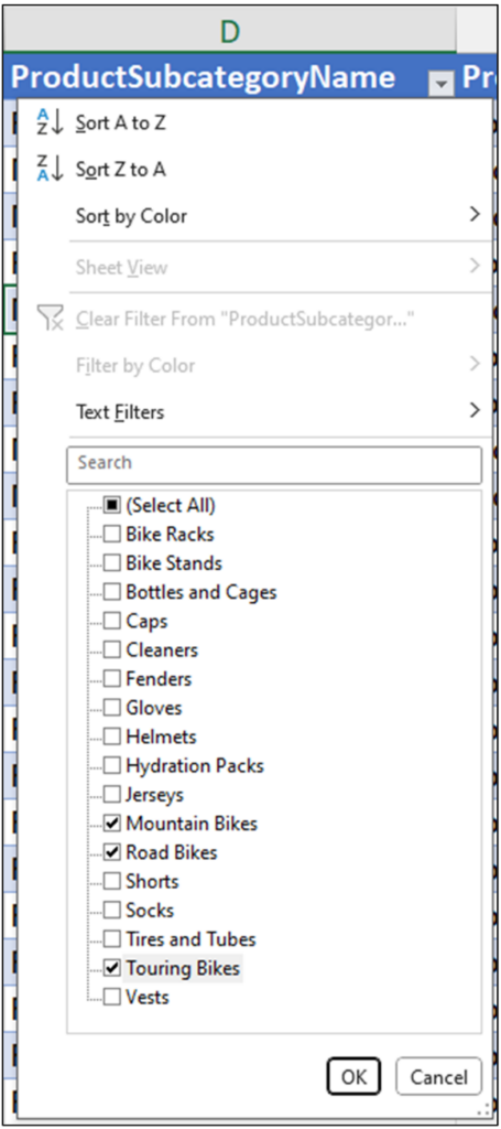
Imagine you wanted to filter the InternetSales table to the rows of data where the ProductSubcategoryName was equal to the value of “Road Bikes.”
Using an Excel table makes defining a filter easy via a graphical user interface (GUI):
Fig 1 – Filtering the InternetSales table using a single value
Clicking OK in the filter GUI applies the filter to the InternetSales table. While Microsoft Excel GUIs are very handy for defining and applying filters, they are not the only method by which a table can be filtered.
For example, you could represent the filter depicted in Fig 1 using text such as the following:
ProductSubcategoryName = “Road Bikes”
Using textual representation like the above for filters is common in programming languages, including Python.
Single Value Filtering with Python
Like Microsoft Excel, the pandas library provides many ways to filter data tables. However, one of the most useful is to use the query() method provided by the pandas DataFrame class.
The query() method allows you to define textual filters and apply them to your data. A new DataFrame containing the filtered data is returned.
The query() method is robust and supports many ways of filtering your DataFrames. This blog post will be an introduction to some of the most common ways to use query(). Check out the online documentation for more information on the query() method.
Here’s an example using query() to filter the InternetSales table.
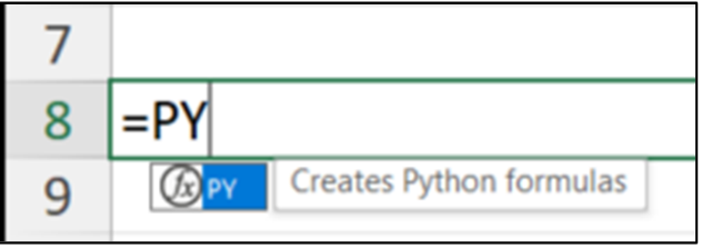
First, use the PY() function to create your Python formula:
Fig 2 – Calling the Excel PY() function
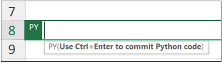
Next, when you type the “(“ the cell will indicate it contains Python code:
Fig 3 – An Excel Python cell
The following Python code implements the filter:
Fig 4 – Calling the query() method to filter the internet_sales DataFrame
Here’s how the above Python code works step by step:
The query() method is called on the internet_sales DataFrame object.
A Python string is used to define the filter.
The filter is defined as only rows of the DataFrame where the ProductSubcategoryName column values are “Road Bikes” within the filter string.
The filtered data is returned as a new DataFrame that is stored in the road_bikes variable.
When looking at the filter used in Fig 4, a few things are worthy of note:
In Python, you use a double equals (i.e., ==) to check for the equivalence of values. This is different from Excel code.
Per Python coding convention, strings are denoted by single quotes. The entire filter string in Fig 4 is wrapped in single quotes.
Because the entire filter string is wrapped in single quotes, you must use double quotes to define the string value of “Road Bikes.”
Hitting <Ctrl+Enter> on your keyboard runs the Python code and produces the output:
Fig 5 – Python code output for Fig 4
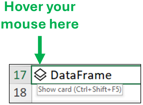
To see the filtered data frame, hover over the card using your mouse:
Fig 6 – Hovering your mouse over the card
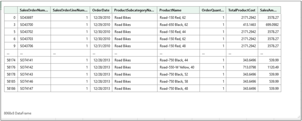
Clicking the card will display the contents of road_bikes:
Fig 7 – The card for the road_bikes DataFrame
As illustrated by Fig 7, the road_bikes DataFrame contains only rows of data for road bikes.
Multi-Value Filtering
Now imagine you wanted to filter the InternetSales table to the rows of data where the ProductSubcategoryName was equal to the value of “Road Bikes,” “Mountain Bikes,” or “Touring Bikes.”
Using the Excel GUI, you can define and apply the filter:
Fig 8 – Filtering InternetSales table using multiple values
The above Excel filter can be represented using text such as the following:
ProductSubcategoryName = “Mountain Bikes” or ProductSubcategoryName = “Road Bikes” or ProductSubcategoryName = “Touring Bikes”
A more succinct textual version of the Excel filter is:
ProductSubcategoryName in (“Mountain Bikes”, “Road Bikes”, “Touring Bikes”)
As you’ve probably guessed, Python code looks very much like the textual filters above.
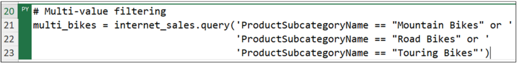
Multi-Value Filtering in Python
Here’s how you define a multi-value filter using the query() method using “or”:
Fig 9 – Calling query() with a multi-value filter using “or”
Note: The above Python code uses multiple strings, each surrounded by single quotes, to allow the code to be broken across multiple lines. This increases the readability of the code.
While you can build multi-value filters by chaining together “or,” it is typically much easier to use “in.” The following Python code is equivalent to the code of Fig 9:
Fig 10 – Calling query() with a multi-value filter using “in”
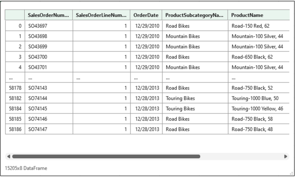
Executing either of the above Python formulas will produce a DataFrame named multi_bikes. If you click on the card for multi_bikes you will see the following:
Fig 11 – The card for the multi_bikes DataFrame
As illustrated by Fig 11, the multi_bikes DataFrame only contains mountain, road, and touring bike data.
Multi-Column Filtering
The InternetSales table is currently being filtered to the rows of data where the ProductSubcategoryName is equal to the value of “Road Bikes,” “Mountain Bikes,” or “Touring Bikes.”
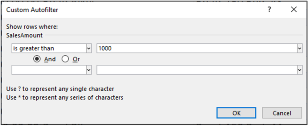
If you want to add a second filter where the SalesAmount value is greater than $1,000, the Microsoft Excel GUI makes that simple:
Fig 12 – Adding a numeric filter to the SalesAmount column
This new filter can be represented textually as follows:
SalesAmount > 1000
When applying filters on multiple columns simultaneously in Excel, you are increasing the complexity of the filter. Excel will automatically return only the rows of the table where both filters are true simultaneously.
In this case, the first filter must be true:
ProductSubcategoryName in (“Mountain Bikes”, “Road Bikes”, “Touring Bikes”)
And the second filter must be true:
SalesAmount > 1000
These two filtering conditions can be combined using the following textual representation:
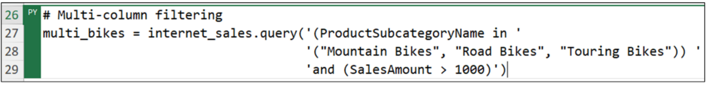
(ProductSubcategoryName in (“Mountain Bikes”, “Road Bikes”, “Touring Bikes”)) and (SalesAmount > 1000)
In the text above, each condition is wrapped in parentheses to ensure each filter condition is evaluated separately.
Multi-Column Filtering in Python
The following Python code implements a filter using the query() method that adds a numeric condition for the SalesAmount column:
Fig 13 – Calling query() with a multi-column filter using “and”
Executing the Python formula above produces a new version of the multi_bikes DataFrame. Clicking on the multi_bikes card displays the following:
Fig 14 – The card for the multi_bikes DataFrame
As illustrated by Fig 14, the multi_bikes DataFrame contains the intersection of the two filtering conditions—just like applying multiple Microsoft Excel filters to a table.
In this post you’ve learned the building blocks for creating DataFrame filters. Using combinations of “or,” “in,” and “and” you can construct complex filters that allow you to select only the rows of data you need for your analysis.
What’s Next?
This blog post has been a brief introduction to filtering pandas DataFrames.
The pandas DataFrame class offers comparable functionality to Microsoft Excel for filtering tables. In addition, using Python code provides benefits in terms of flexibility and reproducibility.
The next post in this series will introduce you to one of the differentiating factors in crafting the best data analyses: cleaning and wrangling your data. Python provides you with two significant advantages in this regard:
Data wrangling techniques that are needed for advanced analytics like machine learning
Standardizing your wrangling process so others can quickly reproduce it
Disclaimer: The Python integration in Microsoft Excel is in Beta Testing as of the publication of this article. Features and functions are likely to change. Don’t hesitate to reach out if you notice an error on this page.
Bio
Dave Langer founded Dave on Data, where he delivers training designed for any professional to develop data analysis skills. Over the years, Dave has trained thousands of professionals. Previously, Dave delivered insights that drove business strategy at Schedulicity, Data Science Dojo, and Microsoft.