Python for Excel Analysts: Data Cleaning and Wrangling

This is the fourth in a series of blog posts that teaches you how to work with tables of data using Python code. The subject of this post is one of the most critical operations in data analysis: cleaning and wrangling your data. 

In case you’re not familiar, here’s a definition from Wikipedia:

“Data wrangling, sometimes referred to as data munging, is the process of transforming and mapping data from one ‘raw’ data form into another format with the intent of making it more appropriate and valuable for a variety of downstream purposes such as analytics.”

As an Excel analyst, you’ve undoubtedly wrangled data many times. Wrangling data is how you get the raw materials for the most impactful data analyses. 

Cleaning and wrangling your data using the Python pandas library provides you with two big advantages: 

• Data wrangling techniques that are needed for advanced analytics like machine learning
• Standardizing your wrangling process so others can quickly reproduce it

If you’re unfamiliar with the pandas library, check out Part 1: The Basics of this blog series.

Each post in this series has an accompanying Microsoft Excel workbook to download and use to build your skills. This post’s workbook is available for download here.

For convenience, here are links to all the blog posts in this series:

• Part 1 – The Basics
• Part 2 – Working with Columns
• Part 3 – Filtering Tables 
• Part 4 – Data Cleaning and Wrangling (this post)
• Part 5 – Combining Tables

Note: To reproduce the examples in this post, install the Python in Excel trial. If you like this blog series, check out my Anaconda-certified course, Data Analysis with Python in Excel.

Adding Columns

One of the most common forms of data wrangling is adding new columns created from data in one or more existing table columns. Examples of this kind of data wrangling include:

• Performing a calculation (e.g., subtracting one column from another)
• Extracting substrings from a column of strings
• Creating a binary indicator (e.g., data was initially missing)

The purpose of adding columns is to increase the usefulness of the data for a particular analytical technique. 

For example, in machine learning, this process is called “feature engineering.” Feature engineering aims to create data representations that are most useful for crafting predictive models.

Adding Columns in Excel

The InternetSales table provides two columns regarding the financial aspect of a sales order: TotalProductCost and SalesAmount. Adding a new column (GrossProfit) would provide additional information useful in many analyses.

The process of adding a new column using Microsoft Excel is straightforward:

With the GrossProfit column created, it needs to be populated with data. The values of GrossProfit should be calculated by subtracting TotalProductCost from SalesAmount for each row in the table.

The most common way Excel users would populate the GrossProfit column is by using a cell reference formula:

Microsoft Excel also supports the use of structured references. For example, the GrossProfit column could be populated using a formula based on the structured references of the TotalProductCost and SalesAmount columns:

Using the formula of Fig 3 and hitting the <enter> key automatically populates the formula for every row of the InternetSales table:

Adding columns to pandas DataFrames is conceptually similar to using Microsoft Excel structured reference formulas.

Adding Columns with Python

Here’s an example of how to add the GrossProfit column to the InternetSales table:

First, use the PY() function to create your Python formula:

Next, when you type the “(“ the cell will indicate it contains Python code:

The following Python code adds the GrossProfit column populated with the calculated values for every row of the internet_sales DataFrame:

Note: The code depicted in Fig 7 appears on multiple lines because the cell is set to Wrap Text using the Excel ribbon.

Conceptually, the code of Fig 7 works like this:

1. The code internet_sales[‘GrossProfit’] tells the internet_sales DataFrame that you want to access the GrossProfit column.
2. As the GrossProfit column does not exist for the internet_sales DataFrame, the equals sign is interpreted as creating a new column.
3. The code to the right of the equals sign is applied row by row.
4. GrossProfit is populated with the computed value of SalesAmount minus TotalProductCost for each row.

Hitting <Ctrl+Enter> on your keyboard executes the Python formula, producing the following in the Excel worksheet:

As nothing was returned from the Python code of Fig 7 (i.e., the code altered the internet_sales DataFrame), the NoneType depicted in Fig 8 is expected.

Running the following Python code will allow you to inspect the altered DataFrame:

To see the altered DataFrame, hover over the card using your mouse:

Clicking the card will display the contents of internet_sales:

As depicted in Fig 11, the Python code produces the same output as the Excel structured reference formula from Fig 3.

Consider the code from Fig 7. When this code is executed, the calculation is automatically performed row by row. This is a behavior of pandas DataFrames known as “vectorization.” 

As an Excel Analyst, you are familiar with vectorization: it’s the default behavior of Excel tables. The support for vectorization with pandas DataFrames makes working with data tables in Python very easy.

Cleaning Data in Python

The previous section covered one of the most common data-wrangling scenarios: adding new columns. This section will cover another common data-wrangling scenario: cleaning the data in an existing column.

Conceptually, cleaning data consists of three steps:

1. Identifying columns that need to be cleaned
2. For columns that need cleaning, performing various cleaning operations
3. Overwriting the original column data with the cleaned data for columns that need cleaning

The quickest way to identify columns needing cleaning is to get a summary of a DataFrame.

DataFrame Summary

DataFrames offer the info() method to provide you with a summary of the DataFrame’s contents:

Executing the code of Fig 12 returns nothing. Instead, calling the info() method will trigger Excel to open the Diagnostics pane to display the DataFrame summary: 

The info() method provides helpful information for identifying columns that need cleaning. Looking at Fig 13, the following information is provided to you:

• There are 60,398 entries (i.e., rows) in the DataFrame.
• There are nine columns in the DataFrame.
• Every column has 60,398 non-null values.
• The following columns are numeric: SalesOrderLineNumber, OrderQuantity, TotalProductCost, SalesAmount, and GrossProfit.
• The OrderDate column is a date-time.
• The following columns are strings: SalesOrderNumber, ProductSubcategoryName, and ProductName

One of the first things you want to identify is if there are any missing values. In most analyses, missing data must be cleaned (e.g., replaced with a default value).

In the info() method output, missing data is represented as null. As each of the DataFrame columns has the same exact count of non-null values as there are rows, no data is missing.

The next step is to profile your numeric and string data.

Profiling Numeric Data

As there is no missing data in the numeric columns of the internet_sales DataFrame, you want to determine if the numeric values are appropriate given the business process.

As detailed in Part 2 of this blog series, the quickest way of profiling numeric data is using the describe() method of a pandas Series (i.e., column). 

DataFrames also have a describe() method that you can use:

The DataFrame describe() method returns a DataFrame containing the profiling details. Clicking on the card in the formula cell displays the profiling results:

Using the information depicted in Fig 15, you can quickly answer the following questions:

• Are there any min/max values that don’t make sense for the business process?
• Does the spread (i.e., distribution) of values make sense for the business process?

Answers to the above questions identify columns that might require data cleaning (e.g., replacing extreme values or removing rows with extreme values).

For example, the OrderQuantity column only contains the value of 1. Depending on the business process, this might be expected or indicate a data quality issue.

Profiling String Data

Columns of string data very often need to be cleaned—especially when the data is entered by humans (e.g., street addresses).

In terms of profiling string data, the value_counts() method of the pandas Series (i.e., columns) is your go-to for understanding string data values:

The value_counts() method returns a Series. The returned Series object contains counts of the unique string values contained within the column. The count values are listed in descending order by default. 

Clicking on the formula cells’ card displays the Series data:

As depicted in Fig 17, pandas DataFrame and Series objects display the first five and last five rows by default. 

This isn’t super useful in this scenario, so an alternative is to tell Excel to return the entirety of the Series data directly to the worksheet as an Excel Value:

Changing the Python formula cell output generates many rows of data:

Fig 19 depicts a common scenario in cleaning string data: specific formatting is used. For example, the various types of bicycles (e.g., “Mountain-100 Black, 42”) follow a formatting of model, color, and size.

A typical data cleaning operation is to transform these string formats.

Cleaning Data

Let’s say you are interested in performing analyses on bicycle sales, but bicycle color isn’t a factor. The current formatting of the ProductName column includes color which will make these analyses difficult.

Cleaning the ProductName column to remove color will allow you to conduct the necessary analyses. As demonstrated in Part 2 of this blog series, the easiest way to achieve this goal is by using the replace() method on the ProductName string column:

Note: The code depicted in Fig 20 appears on multiple lines because the cell is set to Wrap Text using the Excel ribbon.

The easiest way to see the results of the data cleaning is to again use the value_counts() method, with the Series object output returned to the worksheet as an Excel Value:

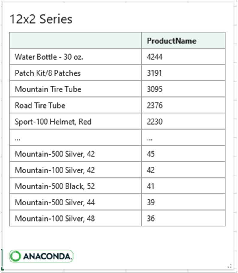
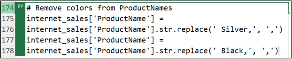
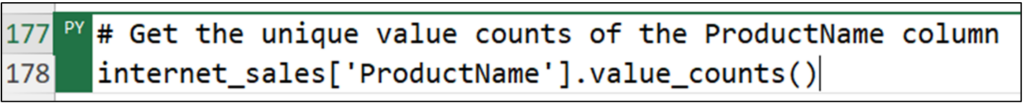
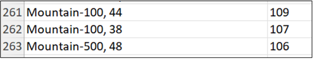
Fig 22 depicts how the cleaned ProductName data can now be used to analyze bicycle sales independent of bicycle color.

The pandas Series data type offers an extensive library for working with string data. Check out the online documentation for more information.

Note: The data cleaning example used in this post is common, but certainly not the only way to clean data. For more resources on data cleaning, check out these Anaconda courses: Introduction to pandas for Data Analysis and Data Cleaning with pandas.

What’s Next?

This blog post has been a brief introduction to data wrangling using pandas.

The pandas library offers a tremendous amount of capabilities for cleaning and wrangling data. This includes all the functionality you’ve used in Microsoft Excel in the past, and much more. 

It is common for the bulk of data analysis Python code to be focused on acquiring, cleaning, and wrangling data. Building Python data-wrangling skills will serve you well.

The last post in this series will introduce you to another essential operation in crafting the best data analyses: joining tables of data (think VLOOKUP). Using Python to join tables of data provides you with three significant advantages in this regard:

• A complete set of various table join operations commonly used to prepare data for advanced analytics
• A greater level of control over how tables of data are joined
• Standardizing your joining logic so others can quickly reproduce it

If you want to learn more about working with data tables using pandas, take a beginner course for an Introduction to pandas for Data Analysis, and check out the official pandas user guide.

Disclaimer: The Python integration in Microsoft Excel is in Beta Testing as of the publication of this article. Features and functions are likely to change. Don’t hesitate to reach out if you notice an error on this page.

Bio

Dave Langer founded Dave on Data, where he delivers training designed for any professional to develop data analysis skills. Over the years, Dave has trained thousands of professionals. Previously, Dave delivered insights that drove business strategy at Schedulicity, Data Science Dojo, and Microsoft.