Introduction to Text Analysis with Python in Excel

Text analysis is an essential technique for extracting valuable insights from unstructured text data that serves as a fundamental component of natural language processing (NLP) applications and more. In this blog post, we will explore an exciting new way to perform text analysis using Python within the familiar environment of Microsoft Excel, made possible by the powerful Anaconda Distribution for Python. This cutting-edge functionality brings together the strengths of Python’s data analysis capabilities and the user-friendly interface of Excel, unlocking a whole new realm of opportunities for efficient and effective text analysis.

Note: To reproduce the examples in this post, install the Python in Excel trial. 

Read in Data

The first step of text analysis is to import the textual data into our Python environment. We can use familiar libraries like pandas to read data directly from Excel. In this example, we have a collection of 20 course reviews stored in the “data” workbook. In a separate sheet, we can start writing Python code by simply entering “=py.” This allows us to access the data with df=xl(“data!A1:A20”, headers=True), which results in a Python DataFrame object. 

Next, to verify that we have loaded the data correctly, we can start another Python environment with “=py” and check the first five rows of data using “df.head().” This quick and straightforward step allows us to ensure the data has been successfully imported and offers a glimpse into the initial records for further analysis.

Define Stop Words

During text analysis it is common practice to filter out stop words, which are frequently occurring words that lack substantial contextual meaning in a sentence (e.g., “a,” “the,” “and,” “but,” etc.). By eliminating these nonessential words, we can focus on the more relevant content and gain more meaningful insights from the text data. We often use the Natural Language Toolkit (NLTK) library to download a list of stop words:

from nltk.corpus import stopwords
stopwords_list = stopwords.words('english')

However, the current version of Python in Excel does not allow you to download the datasets generally required by NLTK. While we’re waiting for resolution, we can define our own list of stop words directly within the code. In the code below, we’ve simply copied and pasted all the stop words from NLTK. Feel free to define a list of stop words on your own to experiment and see how they can impact results. 

N-Gram Analysis

N-grams are contiguous sequences of words from a given sample of text. N-gram analysis is useful for understanding the relationships between words and identifying frequently occurring phrases. In this section, we will investigate combinations of two words and three words, or bigrams and trigrams.

We’ll use the CountVectorizer function, which allows us to convert a collection of text documents into a matrix of token counts. The ngram_range parameter defines the lower and upper boundaries of the range of n-values for different n-grams to be extracted. In this example, we are interested in bigrams and trigrams. The following code snippet illustrates how to obtain all the bigrams and trigrams, sort them by their respective frequencies, and return the top 10 bigrams/trigrams:

from sklearn.feature_extraction.text import CountVectorizer

# Create CountVectorizer object
# CountVectorizer converts a collection of text documents to a matrix of token counts
c_vec = CountVectorizer(stop_words=stopwords_list, ngram_range=(2,3))
# Fit the CountVectorizer to the reviews data to get a matrix of ngrams
ngrams = c_vec.fit_transform(df['reviews'])
# Count the frequency of ngrams
count_values = ngrams.toarray().sum(axis=0)
# Get a list of ngrams
vocab = c_vec.vocabulary_
# Create a DataFrame to store the frequency and n-gram, sorted in descending order of frequency
df_ngram = pd.DataFrame(sorted([(count_values[i],k) for k,i in vocab.items()], reverse=True)
            ).rename(columns={0: 'frequency', 1:'bigram/trigram'})
# Display the top 10 n-grams by frequency
df_ngram.head(n=10) 

The analysis reveals that the phrase “textbook great” appeared six times, while “assignments hard” was found four times in the text data. These frequent occurrences of specific word combinations offer valuable insights into the patterns in the analyzed text.

Topic Modeling

Topic modeling is a technique used to discover the main topics or themes within a collection of documents. It helps to organize text data and provides a concise representation of the underlying information. There are two main models for topic modeling: Non-Negative Matrix Factorization (NMF) models and Latent Dirichlet Allocation (LDA) models. In this example, we will use the NMF method. 

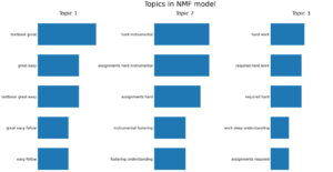
NMF is an unsupervised technique that can reduce the dimension of input data. More specifically, it is a powerful matrix decomposition procedure that breaks a matrix into the product of two non-negative matrices: W and H. By default, NMF optimizes the distance between the original matrix and WH. Below is an illustrative example wherein we apply NMF to generate three topics and showcase five significant bigrams/trigrams within each topic.

from sklearn.feature_extraction.text import TfidfVectorizer
from sklearn.decomposition import NMF
from sklearn.pipeline import make_pipeline

# Create a TF-IDF vectorizer object
# TF-IDF (Term Frequency-Inverse Document Frequency) is a technique used to quantify a word in documents
# It is used to reflect how important a word is to a document in a collection or corpus
# The stop_words parameter is used to ignore common words in English such as 'this', 'is', etc.
# The ngram_range parameter is used to specify the size of word chunks to consider as features
tfidf_vectorizer = TfidfVectorizer(stop_words=stopwords_list, ngram_range=(2,3))

# Create an NMF (Non-Negative Matrix Factorization) object
# The n_components parameter is used to specify the number of topics to extract
nmf = NMF(n_components=3)

# Create a pipeline object that sequentially applies the TF-IDF vectorizer and NMF
pipe = make_pipeline(tfidf_vectorizer, nmf)

# Fit the pipeline to the reviews data
pipe.fit(df['reviews'])

def plot_top_words(model, feature_names, n_top_words, title):
    """
    Plot top words in topics 
    source: https://scikit-learn.org/stable/auto_examples/applications/plot_topics_extraction_with_nmf_lda.html#sphx-glr-auto-examples-applications-plot-topics-extraction-with-nmf-lda-py
    """
    import matplotlib.pyplot as plt
    fig, axes = plt.subplots(1, 3, figsize=(30, 15), sharex=True)
    axes = axes.flatten()
    for topic_idx, topic in enumerate(model.components_):
        top_features_ind = topic.argsort()[: -n_top_words - 1 : -1]
        top_features = [feature_names[i] for i in top_features_ind]
        weights = topic[top_features_ind]

        ax = axes[topic_idx]
        ax.barh(top_features, weights, height=0.7)
        ax.set_title(f"Topic {topic_idx +1}", fontdict={"fontsize": 30})
        ax.invert_yaxis()
        ax.tick_params(axis="both", which="major", labelsize=20)
        for i in "top right left".split():
            ax.spines[i].set_visible(False)
        fig.suptitle(title, fontsize=40)

    plt.subplots_adjust(top=0.90, bottom=0.05, wspace=0.90, hspace=0.3)
    plt.show()

# Plot the top words in the topics identified by the NMF model
plot_top_words(
    nmf, tfidf_vectorizer.get_feature_names_out(), 5, "Topics in NMF model"
)

The analysis yielded the following insights:

• Topic 1: Focuses on the theme of a “great textbook”
• Topic 2: Highlights the challenges posed by “hard assignments”
• Topic 3: Emphasizes the importance of “hard work”

These findings offer valuable clarity on the main topics within the course reviews. 

Conclusion

Text analysis is a valuable tool that can provide meaningful insights from unstructured text data. In this blog post, we covered the basics of text analysis, including n-gram analysis and topic modeling, using Python in Excel. By leveraging this new integration of Python’s libraries, you can perform analyses that were not previously possible within the familiar interface of Excel. Additionally, you can easily share valuable results with stakeholders directly within Excel, where they are already comfortable working.

Disclaimer: The Python integration in Microsoft Excel is in Beta Testing as of the publication of this article. Features and functions are likely to change. Don’t hesitate to reach out if you notice an error on this page. 

Bio

Sophia Yang is a Senior Data Scientist and a Developer Advocate at Anaconda. She is passionate about the data science community and the Python open-source community. She is the author of multiple Python open-source libraries such as condastats, cranlogs, PyPowerUp, intake-stripe, and intake-salesforce. She serves on the Steering Committee and the Code of Conduct Committee of the Python open-source visualization system HoloViz. She also volunteers at NumFOCUS, PyData, and SciPy conferences. She holds an M.S. in Computer Science, an M.S. in Statistics, and a Ph.D. in Educational Psychology from The University of Texas at Austin.