Understanding Python data structures might seem purely academic—until you’re processing millions of records and your code takes hours instead of minutes. The structure you choose determines whether operations take constant time or scale linearly with data size.
Working with a large numerical dataset? NumPy arrays can deliver 10-100x performance improvements over lists. Need fast lookups? Dictionaries can provide millisecond access times for multimillion-record searches, whereas lists can take several minutes.
For developers working with large datasets in the Python programming language, it’s crucial to understand how structures operate in different scenarios. This tutorial covers which structures to use when, how they perform at scale, and how to reliably implement them.
What are Python Data Structures?
Data structures are organized formats for efficiently storing, accessing, and manipulating data in computer memory. In Python, they range from built-in types (like lists and dictionaries) to specialized implementations in libraries (like NumPy and pandas.) Each structure offers different trade-offs between access speed, memory usage, and operational complexity. Recognizing those trade-offs is crucial for writing efficient code.
Why Data Structures Matter in Python
Python’s main built-in data structures (lists, tuples, dictionaries, and sets) handle most everyday programming tasks. These are distinct from abstract data structures—computer science concepts like stacks, queues, and trees that serve as building blocks for more complex programs. You can implement these using Python’s built-in types or specialized libraries.
The structure you choose directly impacts:
- Performance (how fast operations execute)
- Memory usage (how much RAM your data consumes)
- Scalability (how performance changes as data grows)
These factors matter most when working at scale, such as processing datasets that approach your system’s memory limits or running operations millions of times, which can cause small inefficiencies to compound.
Want hands-on practice? Anaconda’s Python Data Structures and Algorithms course provides interactive tutorials and coding exercises to deepen your understanding of these concepts.
Categories of Data Structures
Data structures fall into two broad categories that organize data in fundamentally different ways.
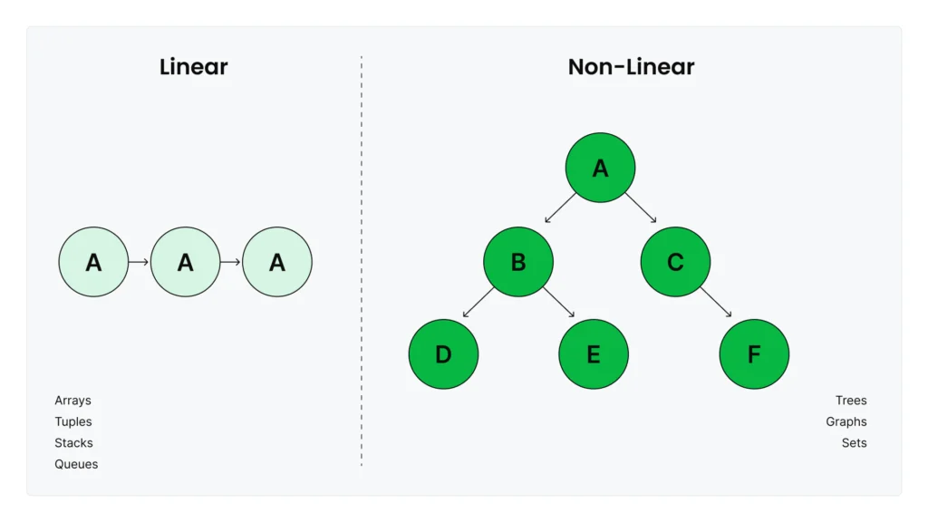
Linear structures like lists, tuples, and arrays preserve the order of elements as you add them. Stacks and queues are also linear structures, which you can implement using lists or the collections.deque class. They’re ideal when you need to process data in order, maintain sequences, or access elements by position.
Non-linear structures organize data in hierarchical or networked relationships where elements can connect to multiple others. Trees, graphs, and hash tables (like Python’s dictionaries) fall into this category. They excel at representing complex relationships—like social networks, knowledge graphs, or fast key-value lookups—that don’t fit into simple sequential patterns.
Linear Data Structures in Python
Lists and Arrays
A list is a collection of items that stores any type of Python object and automatically resizes as you append or remove elements. You can create lists using square brackets: my_list = [1, 2, 3], or start with an empty list []. They’re iterable, which means you can loop through their elements sequentially. They’re also mutable, which means you can modify, append, or remove elements after creation. This flexibility makes them ideal for small collections or mixed data types, but it creates performance limitations for large numerical datasets.
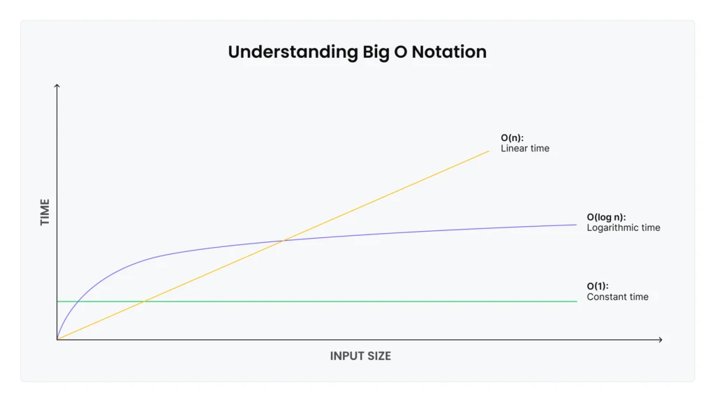
List performance characteristics: Appending or removing items at the end of a list is fast—it takes the same amount of time regardless of list size. But appending or removing items at the beginning or middle is slow, since Python has to shift all subsequent elements. For a list with 1 million items, removing the first element means shifting 999,999 items to new positions in memory.
Computer scientists describe these performance characteristics using Big O notation: Operations that stay fast regardless of size are O(1) (constant time), while operations that slow proportionally to the number of elements are O(n) (linear time). Appending items to the end of the list is O(1), while inserting items at the beginning or middle is O(n).
When you’re working with large numeric datasets in machine learning (ML) pipelines, lists can quickly become a bottleneck. That’s where NumPy arrays excel.
Why NumPy arrays matter for ML: NumPy arrays are specialized structures optimized for numerical computation. Unlike Python lists, which store each element as a separate Python object with type information and metadata, NumPy arrays store raw numeric data in contiguous memory blocks with all elements as the same data type. For numeric data, NumPy arrays use significantly less memory—typically 3-5x reduction compared to Python lists. A list holding 1 million floats (decimal numbers) might consume 20+ MB, while a NumPy array holding the same data fits in 4 MB.
The real performance advantage comes from vectorization. NumPy operations are implemented in compiled C code and use the SIMD (Single Instruction, Multiple Data) capabilities of modern CPUs, which allow the processor to perform operations on multiple array elements at once. Benchmarks show NumPy can be up to 25x faster at creating arrays, up to 200x faster for arithmetic operations, and up to 22x faster for aggregations compared to equivalent list operations. For element-wise operations on 1 million elements or more, NumPy can deliver 10-100x speedup.
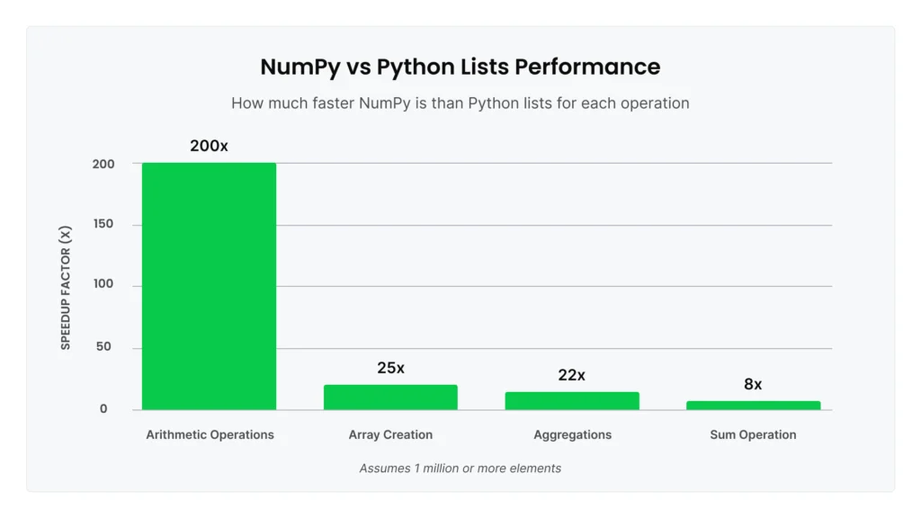
Here’s a concrete example: Summing 1 million numbers. With Python’s built-in sum() on a list, this takes significant time due to Python-level iteration. Using NumPy’s optimized np.sum() on an array is at least 8x faster for the same operation.
NumPy’s performance advantages are dramatic for the right use cases, but it’s not universally faster. Knowing when to stick with lists is equally important:
- Small datasets: For small arrays (typically under a few hundred elements), Python lists are simpler and faster.
- Scalar operations: Python’s math library is roughly 10x faster than NumPy for single-value calculations.
- Python-level iteration: If you’re looping through array elements one by one rather than using vectorized operations, NumPy will be slower than lists because each element must be “unboxed” from the array into a Python object.
- Sequential logic: For operations where each step depends on the previous result—like tree traversal or custom conditional logic—Python lists reign supreme.
For the scenarios where NumPy excels (large numerical datasets with vectorized operations), Anaconda’s curated repository provides tested, compatible versions of NumPy and its dependencies, eliminating installation complexity and version conflicts.
To broaden your understanding of Python lists and arrays, refer to this tutorial.
Tuples
Tuples are ordered collections of elements, similar to Python lists. Both store sequences you access by index position. But unlike lists, which are mutable objects you can modify freely, tuples are immutable objects—once created, you cannot change them. This mutability difference can help you determine when to use lists versus tuples.
Here’s a simple tuple storing RGB color values:
color = (255, 128, 0)  # Orange in RGB
red_value = color[0]  # Access by index, returns 255
You create tuples using parentheses syntax: my_tuple = (1, 2, 3), or even without parentheses for simple cases: coords = 10, 20.
Tuple performance characteristics: Because tuples are immutable, they’re slightly more memory-efficient than Python lists, and they’re faster to create. Index access is O(1), meaning tuples have the same constant-time performance as lists. You can also iterate through tuples, slice them, and check their length just like lists. The main operations you can’t do are modifications—no appending, inserting, or removing elements.
When to use tuples: Immutability makes tuples ideal for data that shouldn’t change. Use tuples for:
- Fixed data: Coordinates
(x, y), RGB values(255, 128, 0), or database records you want to protect from accidental modification - Dictionary keys: Unlike lists, tuples can serve as dictionary keys because their immutability guarantees the key won’t change
- Function returns: Python functions often return multiple values as tuples:
return (min_value, max_value, average) - Data integrity: When you want to signal “this data is final” or prevent other code from modifying your data structure
For most use cases where you need a collection that grows or changes over time, Python lists are more flexible. But when you need to guarantee data won’t be modified—either for safety, for use as dictionary keys, or to clearly communicate intent—tuples provide that protection.
Want a more comprehensive tutorial on tuples? Follow this tutorial.
Stacks and Queues
Stacks and queues are abstract data structures that restrict how you access elements. This restriction makes stacks and queues especially useful for specific algorithms.
A stack follows Last-In-First-Out (LIFO) ordering, meaning the most recently added element is removed first, like a stack of plates. A queue follows First-In-First-Out (FIFO) ordering, meaning elements are removed in the order they were added, like a line at a coffee shop.
You can implement both data structures using Python lists with append() and pop(). For stacks, this works well, because appending and removing from the end of the list are both O(1) operations. But for queues, lists are inefficient. A queue needs to remove items from the beginning of the list with list.pop(0), which is O(n). For a queue with 10,000 items, every removal operation shifts 9,999 items in memory.
That’s where collections.deque (double-ended queue) becomes essential. Deque provides O(1) operations at both ends of the sequence. Benchmarks show deque.popleft() can be 40,000x faster than list.pop(0) for removing items from the front. If you’re implementing a stack or queue, or you need frequent additions and removals at both ends, deque is dramatically more efficient.
Real use case: When an ML model serves predictions to multiple clients, you need to process requests in the order received. A queue ensures fairness—the first request gets processed first. Using collections.deque provides the O(1) performance needed to handle high request volumes:
from collections import deque

request_queue = deque()
request_queue.append(new_request)  # Add to back: O(1)
next_request = request_queue.popleft()  # Remove from front: O(1)
Learn more about stacks, queues, and priority queues in this tutorial.
Hierarchical and Hashed Data Structures
Dictionaries and Hashed Tables
Dictionaries (often abbreviated as dicts) are among the most powerful built-in data structures in Python. They store data as key-value pairs in an unordered collection. They provide O(1) time complexity for lookups, insertions, updates, and deletions, meaning they take the same amount of time whether you’re working with 100 items or 100 million.
As an example, here’s a simple dictionary storing user ages:
user_ages = {"alice": 28, "bob": 35, "charlie": 42}
age = user_ages["alice"]  # Instant lookup, returns 28
You can create an empty dictionary with {} or dict() and add key-value pairs dynamically.
How dicts stay fast: When you access user_ages["alice"], Python doesn’t search through all keys. Instead, it computes a hash value (a number) from the key “alice” and uses that to jump directly to the value’s location in memory, much like using a phone book’s alphabetical tabs instead of reading every page. This direct access is why lookups remain fast, even with millions of entries.
Python maintains extra space in hash tables to avoid collisions (when different keys produce the same hash value). Dicts must use unique keys—no duplicates allowed. Each key can appear only once to ensure unambiguous lookups.
When collisions do occur, Python uses a technique called “perturbation probing” to find an alternative location. While the worst case is O(n) if many keys collide, Python’s hash function makes this extremely rare.
Dicts in data science: The O(1) lookup makes dicts ideal for several common patterns.
- Feature lookups: When training ML models, you often need to retrieve pre-computed features for millions of entities (users, products, transactions). Storing these in a dictionary with entity IDs as keys provides instant O(1) access. If you use a list instead, you’ll have to search through all entries for each lookup, turning seconds into hours for large datasets.
- Categorical encoding: When transforming text categories into numbers for ML models, dicts provide the mapping:
{"cat": 0, "dog": 1, "bird": 2}. Looking up “cat” returns 0 instantly, no matter how many categories you have. - Caching expensive calculations: If a function takes five seconds to compute but gets called repeatedly with the same inputs, you should store results in a dict. The first call computes and stores the result, and subsequent calls with the same input can retrieve the cached result in microseconds instead of recomputing. In iterative algorithms, that pattern can reduce runtime from hours to minutes.
Sets
Sets are unordered collections of unique elements implemented using hash tables. They’re similar to dictionaries, but they store only keys without associated values. Like dictionaries, Python sets provide O(1) time complexity for membership testing, insertion, and deletion.
You can create sets using curly braces with elements: my_set = {1, 2, 3} or set() for an empty set. Sets automatically eliminate duplicates, which means adding the same element multiple times results in a single occurrence.
When to use sets: The primary use case is fast membership testing. Checking if item in my_set is O(1) regardless of set size, while the same operation on a list is O(n). For a collection of 1 million items, this difference can turn minutes of searching into microseconds.
Sets also excel at deduplication. Converting a list to a set with unique_items = set(my_list) instantly removes all duplicates, which is far more efficient than manually tracking seen elements.
Set operations: Python sets support mathematical set operations that are useful for data analysis, such as:
- Union (
set1 | set2): Combines all unique elements from both sets - Intersection (
set1 & set2): Returns only elements present in both sets - Difference (
set1 - set2): Returns elements in set1 but not in set2
These operations are particularly useful when comparing datasets, finding common elements across groups, or identifying unique values in data pipelines.
Sets in data science: Common patterns include removing duplicate records from datasets before analysis, quickly checking if values exist in large reference lists (like validating user IDs against a set of valid IDs), and finding overlaps between categories (like identifying users who belong to multiple segments).
The main limitation is that sets are unordered. That means you can’t access elements by position or rely on any particular iteration order. If you need both fast membership testing and ordered elements, consider dictionaries or specialized data structures.
Trees and Binary Trees
Trees are branching data structures in Python, similar to a family tree or a company’s org chart. Unlike linked lists which connect elements sequentially, each element in a tree (called a node) can connect to multiple elements below it (called children), creating parent-child relationships.
In machine learning, decision trees are the most common tree structure you’ll encounter. Each node represents a decision rule like “is age > 30?” and the branches lead to different outcomes based on those decisions. When you use a decision tree model to make a prediction, it traverses a path down the tree by checking rules at each node—a process that’s fast even with complex feature sets. Decision trees are also interpretable: You can trace exactly which rules led to a specific prediction.
Algorithms like Random Forest and XGBoost combine multiple decision trees to improve accuracy. These are among the most powerful ML algorithms for tabular data.
For production work, you don’t need to build tree structures yourself. Libraries like scikit-learn, for example, provide highly optimized C implementations that handle all the tree mechanics internally. Still, understanding trees conceptually can help you use these tools effectively and interpret their results.
Graphs and NetworkX
Graphs represent networks of connections between entities. Think of a social network where people (nodes) are connected by friendships (edges), or a knowledge base where concepts link to related concepts.
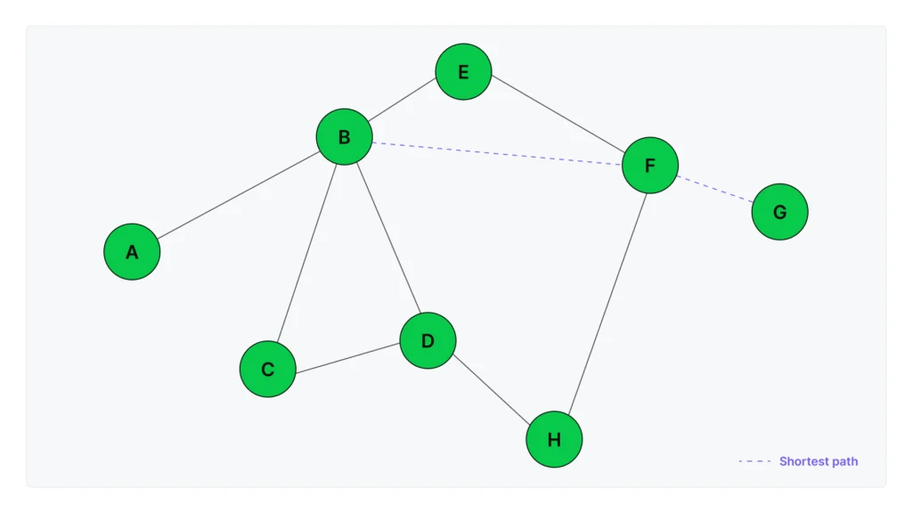
Unlike trees, graphs can have cycles (A connects to B, B connects to C, C connects back to A) and any node can connect to any other node, making them ideal for representing complex real-world relationships.
NetworkX is Python’s primary library for working with graph structures. It provides the data structures and algorithms you need to build, analyze, and visualize networks without implementing graph theory from scratch.
Common NetworkX operations include shortest_path() for finding optimal routes between nodes, centrality algorithms for identifying important nodes in a network, and community detection for finding clusters of closely related nodes.
NetworkX depends on NumPy, SciPy, and Matplotlib for advanced operations and visualizations. Anaconda’s curated repository ensures these packages work together—just install NetworkX with conda install networkx, and all compatible dependencies are automatically resolved.
Graphs in data science: NetworkX enables several powerful patterns for working with connected data.
- Knowledge graphs: Search engines and question-answering systems use knowledge graphs to capture how entities relate to each other. A medical knowledge graph might represent “DrugA treats Disease1” and “Gene2 associated with Disease1” as connected nodes. NetworkX makes it straightforward to build and query these structures for all types of applications, from healthcare analytics to enterprise knowledge management.
- Recommendation systems: Recipe recommendation systems can use a type of graph called bipartite, where one set of nodes represents recipes and another represents ingredients. Edges connect each recipe to its ingredients. NetworkX’s bipartite algorithms identify which recipes share the most ingredients, enabling recommendations like “people who made this recipe also made…” based on ingredient overlap.
- Social network analysis: Friend recommendation features use graph structures to represent connections between people. NetworkX provides algorithms for community detection (finding groups of closely connected users), centrality measures (identifying the most influential users in a network), and link prediction (suggesting new friendships based on mutual connections). These same techniques apply to professional networks, citation networks, and any domain where relationships between entities matter.
- Graph machine learning: Advanced ML techniques can use graph structures as model inputs. Methods like node2vec learn numerical representations of each node based on its position and connections in the network. These representations enable predictions like classifying users based on their connections or predicting missing links in incomplete networks. NetworkX integrates with specialized graph ML libraries for these use cases.
Learn more about making GenAI work with your enterprise data.
Choosing the Right Structure for the Job
Time and Space Tradeoffs
Understanding the performance characteristics of each structure helps you choose the right one for your use case. The table below compares the structures we’ve covered:
This table focuses on the most commonly used structures for data science work. For comprehensive coverage, including tuples and sets (unordered collections of unique elements optimized for membership tests), see the Python documentation.
| Structure | Best for | Access time | Insert/delete | When to use | Avoid for |
|---|---|---|---|---|---|
| List | Mixed types, small collections | O(1) by index | O(n) at start, O(1) at end | Small datasets, heterogeneous data, simple operations | Large numeric computations, frequent insertions at start |
| NumPy array | Numerical operations at scale | O(1) by index | O(n) resize | Large datasets (1,000+ elements), vectorized math | Small datasets, mixed types, element-by-element iteration |
| Dicts | Fast key-value lookups | O(1) by key | O(1) | Feature stores, caching, categorical encoding | Columnar operations or vectorization |
| deque | Operations at both ends | O(1) at ends, O(n) in middle | O(1) at ends | Queues, sliding windows, stacks | Random access in middle |
| DataFrame | Tabular data with mixed types | O(1) by column name | O(1) add column, O(n) for rows | ML pipelines, data with labeled columns, SQL-like operations | Simple numeric arrays (use NumPy instead) |
Use this table as a quick reference when deciding between structures. The key principle is to match your data structure to your access pattern and data characteristics.
Real-World Scenarios
Here’s how these Python data structures apply to real data science and ML workflows.
Feature stores using dictionaries
ML systems often pre-compute features (user demographics, product statistics, transaction history) and store them for quick retrieval during model training. If you store millions of user features in a dictionary with user IDs as keys, you get O(1) lookup time, which means retrieving features for 1 million users stays fast. Using a list would require searching through entries for each lookup, turning what takes seconds with a dictionary into hours with a list.
Queues in ML inference pipelines
When your model provides predictions to multiple clients, you need to process requests fairly (e.g., first request in, first request processed). Using collections.deque as a FIFO queue ensures each request gets handled in order without any client waiting indefinitely. The O(1) operations at both ends mean your queue handles high request volumes without becoming a bottleneck.
Graph structures in recommendations
E-commerce recommendation systems can use graphs where one set of nodes represents users and another represents products. Edges represent interactions like purchases or views. NetworkX can analyze this structure to find patterns like “users who bought this product also bought…” Representing that data in tables would require complex joins and lookups, but the graph structure captures these relationships naturally.
Time-series data using NumPy arrays
Financial data and sensor readings often require rolling window calculations, such as computing moving averages or standard deviations over sliding time periods. NumPy’s vectorized operations turn what would be nested loops (slow) into single function calls (fast). For large time-series datasets, this reduces computation time from minutes to seconds.
DataFrames for feature engineering
When preparing data for ML models, you typically work with mixed data types—numeric features, categorical variables, timestamps, and text. DataFrames let you store all these types together with labeled columns and apply SQL-like operations. For example, grouping customer transactions by user ID and computing aggregate statistics becomes a single df.groupby('user_id').agg(...) call instead of writing loops and managing nested dictionaries.
In production ML workflows, data structure bugs often stem from environment drift—code that worked in development breaks in production because NumPy or pandas was updated. This is especially dangerous for feature engineering pipelines where different array behavior can silently change model inputs. Conda environments prevent this by locking dependencies, which ensures your Python data structure implementations behave consistently across environments.
Tools and Libraries to Help You Work with Data Structures
Built-In Python Libraries
Beyond the basic data structures, Python’s collections module provides enhanced versions for specific use cases:
- Counter: Simplifies counting how many times each item appears in a collection. Instead of manually tracking counts in a dictionary,
Counterdoes this automatically. - defaultdict: Provides default values for keys that don’t exist yet. Useful when counting or grouping data without checking if a key already exists—avoiding ‘key not found’ errors.
- namedtuple: Creates simple data containers with named attributes. Instead of accessing tuple elements by index (
user[0],user[1]), you can use names (user.name,user.age).
These tools are part of the standard Python library, requiring only import collections to use. They’re approachable for beginners while providing powerful functionality for advanced use cases. For detailed usage and more options, see Python’s official collections documentation.
Open-Source Libraries (included in Anaconda)
The data science and data analysis ecosystem relies on specialized libraries—NumPy for numerical arrays, pandas for tabular data, and NetworkX for graphs. Anaconda’s curated repository bundles compatible versions together, so installing with conda install numpy pandas networkx gives you tested combinations that work reliably without manual dependency resolution.
pandas DataFrames as Specialized Data Structures
DataFrames are sophisticated data structures built on NumPy arrays. They store data in columns, with each column internally stored as a NumPy array. Columns of the same data type are grouped together in memory, which is why column operations are fast but row-by-row iteration is slow.
Why DataFrames matter: Unlike NumPy arrays, which require all data to be the same type, DataFrames can mix integers, decimals, text, and dates in different columns—all in one structure. This makes them ideal for typical ML datasets where you have numeric features alongside categorical variables and timestamps. You can also access columns by name (df['age']) rather than numeric index, and use SQL-like operations (groupby, join, merge, pivot) for data transformation.
When to use DataFrames: They’re the primary tool for ML data pipelines. Use them when you need to:
- Transform raw data into features for model training
- Clean and filter datasets with mixed data types
- Group and aggregate data (like calculating average purchase value per customer)
- Prepare data for ML libraries—DataFrames convert easily to NumPy arrays for scikit-learn
Performance tips: Operate on entire columns rather than looping through rows individually. Column operations use vectorized NumPy underneath and stay fast. Row iteration forces Python to process elements one at a time, which is slow. For performance-critical workflows at scale, consider Polars—a DataFrame library that can be significantly faster than pandas for large datasets.
Memory optimization: DataFrames default to 64-bit types for numbers, which can waste memory. Converting to smaller types when possible (64-bit integers to 8-bit for small numbers) can reduce memory usage by 8x. For text columns with repeated values, using the categorical type stores unique values once and uses numeric codes for repetitions, providing massive memory savings. Optimizations like these can reduce DataFrame memory by 60% or more: One case study reduced a DataFrame from 93 MB to 36 MB.
Environment Management with Conda
The Python data structures we’ve reviewed so far all depend on specific library versions. Managing these environments ensures your code behaves consistently across development, testing, and production.
The reason this matters is because different projects often need different package versions. One ML project might require NumPy 1.24 for compatibility with older code, while another needs NumPy 1.26 for new features. Installing different versions of the same package creates conflicts where updating one project breaks another. Team collaboration requires everyone to work with identical environments so performance benchmarks stay consistent. Production deployment demands that dev, staging, and production use exactly the same versions to avoid environment drift.
Conda solves this with isolated environments. Each project gets its own Python version and packages. An environment.yml file captures exact dependencies:
name: data-structures-project
dependencies:
  - python=3.11
  - numpy=1.24.3
  - pandas=2.0.1
  - networkx=3.2
  - jupyter
Share this file via git, and anyone can recreate the identical environment with one command: conda env create -f environment.yml. This ensures cross-platform portability—the same environment works on Windows, macOS, and Linux, and conda resolves platform-specific differences automatically.
Consider a real scenario: Your team is benchmarking data structures for a pipeline optimization. Person A (NumPy 1.24.3, pandas 2.0.1) measures a 150x speedup from switching lists to arrays. Person B (NumPy 1.26.0, pandas 2.2.0) measures 180x speedup. The results aren’t comparable: Is the difference from code changes or library variations? Conda environments lock everyone to the same versions via environment.yml, everyone benchmarks with identical packages, making performance comparisons trustworthy.
To learn more about environment management with conda, refer to this tutorial.
Final Thoughts: Building Scalable, Performant Python Projects
The performance differences we’ve explored determine whether your ML pipelines run in minutes or hours. When you move from development datasets to production volumes, these differences separate code that scales from code that fails.
That’s why choosing Python data structures wisely requires understanding their complexity and managing the tools that implement them. The NumPy arrays you benchmark in development need to behave identically in production, and your team’s performance testing needs identical package versions to produce comparable results.
Anaconda addresses both challenges. Our curated repository provides tested combinations of Python packages that work reliably together, eliminating dependency conflicts. And because conda’s environment management locks package versions across development, testing, and production, your code behaves consistently everywhere.
Ready to apply these concepts? Get started with Anaconda Distribution at anaconda.com/download.