Introduction
In this blog, we will do a walk-through of implementing a complete machine learning (ML) lifecycle on AWS-Graviton-based Amazon EC2 instances (AWS Graviton for short from now on) for a real-world fraud detection dataset use case. This is an example, and you can use Anaconda Distribution on AWS Graviton to work on various kinds of ML use cases. The takeaways after reading this blog are as follows:
- AWS Graviton can be used for doing training and inferencing on classical ML workloads and inferencing for deep learning workloads. CPUs in general offer ease of use in terms of debuggability with minimal need for learning something new. All the details for running ML workloads on arm64 processors are abstracted away. In addition, Graviton can typically deliver better performance than comparable x86-based Amazon EC2 instances. We will use a real-world example of a fraud dataset to showcase this, using decision trees and random forest as classifiers.
- Anaconda Distribution provides immediate access to all the packages to execute and reproduce complete ML workloads, with necessary package support for arm64-based AWS Graviton.
All major machine learning frameworks such as PyTorch, TensorFlow, XGBoost, scikit-learn, etc. are supported on AWS Graviton, which typically offers 40% price-performance and 20% performance benefits over comparable x86-based instances. In addition, Graviton is generally around 60% more energy efficient and hence offers sustainability benefits over comparable x86-based instances.
Anaconda Distribution
Anaconda Distribution is a leading platform in the ML ecosystem, and the world’s most trusted Python distribution. Powering everything from AI solutions to interactive visualizations, Anaconda is the preferred distribution for numerical and scientific computing, providing necessary access to a wide variety of packages and frameworks for data science and machine learning including NumPy, pandas, scikit-learn, PyTorch, and TensorFlow. Anaconda Distribution also pairs with conda to provide simplified package and environment management. Conda environments guarantee full reproducibility of the Python ecosystem across multiple platforms and hardware architectures. Anaconda Distribution support for AWS Graviton started in 2021, and AWS Graviton has reached full support of packages on Anaconda.
ML Lifecycle on AWS Graviton
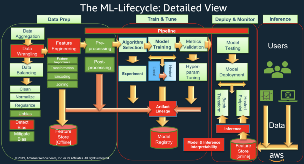
We will showcase how to conduct a complete ML lifecycle on AWS Graviton for an ML business use case of credit card fraud detection. We will demonstrate the support for packages as well as the ease of use on AWS Graviton, similar to x86-based instances for ML workloads. Fig. 2 below shows the various pipeline stages of an ML-lifecycle pipeline. We will focus on the “Data Prep,” “Train & Tune,” and observing model performance parts of the ML lifecycle below. The heavy lifting of performance tuning the underlying ML frameworks for arm64-based AWS Graviton (for example: some of the optimizations for PyTorch 2.0 as listed under “Optimization details”) is done by AWS and abstracted from your code. As you can see, the ML lifecycle has a lot of stages and is an end-to-end way of creating and deploying an ML model. A full ML software stack can be implemented on AWS Graviton using commonly used ML frameworks and Anaconda Distribution.
Credit Card Fraud Detection Use Case Using Anaconda Distribution on AWS Graviton
Scenario
We will be looking at a real-world scenario using a credit card fraud detection dataset from Kaggle. We will train a model to detect fraud using a decision tree package from scikit-learn. Though the dataset is a fraud detection dataset, most of the techniques discussed have broad applicability.
This dataset has been chosen because it represents a good candidate for real-world data challenges in enabling the implementation of a complete and extensive data science and machine learning pipeline.
As is generally the case for fraud detection, the problem at hand can be considered an “anomaly detection” problem. In other words, we should be expecting to deal with a dataset that will be highly skewed towards non-fraud use cases. As a matter of fact, this is the case for our dataset, in which 99.8% of the transactions are non fraudulent and only 0.17% of the transactions included in the dataset reflect fraud.
Setup
We will use Anaconda Distribution for AWS Graviton, following the instructions available in the official documentation. Anaconda Distribution provides automatic guarantees of full reproducibility (in terms of packages and versions) across multiple architectures. This will be crucial for the last section of this post where we will be comparing AWS-Graviton-based instance performance with x86-based instances. As per ML model deployment, on AWS you can use either SageMaker to deploy your models or use self-managed ML. We will showcase self-managed ML on Graviton. There is another blog post that discusses using SageMaker for Graviton.
All of the packages featured in this blog and used throughout the experiments are already part of Anaconda Distribution. For the performance comparison against x86-based instances we will also leverage conda environments created through Anaconda. The key advantage provided by conda environments is full portability of the packages and Python interpreter across all the AWS instances. This allows us to reproduce our environments on three Amazon EC2 (c6i.8xlarge) and AWS-Graviton-based (c7g.8xlarge, c6g.8xlarge) instances. We will be using three AWS EC2 instances running Amazon Linux 2 (AL2) for comparison. This works well for performance comparison to make sure the ML software stack remains the same across multiple benchmarking runs on multiple AWS EC2 instances.
Data Preparation
Commonly used techniques and libraries for data preparation such as NumPy, pandas, and scikit-learn are supported on AWS Graviton via Anaconda Distribution. You don’t need to learn any new libraries or techniques for arm64. Let us start by visualizing the dataset to understand the nature of the data.
The credit card fraud data set consists of 30 features. Besides the “Time” and “Amount” features, all the other feature names are anonymized to preserve privacy. There are a total of 284, 817 transactions (rows) in the dataset. The dataset is pretty clean, with no “Null” values, etc., and the description of the data says that all the anonymized “Vx” features are numerical as a result of principal component analysis (PCA) transformation. The features “Time” and “Amount” were not transformed as per the description of the dataset. Feature “Class” is the response variable and it takes value 1 in case of fraud and 0 otherwise. Some features such as “Time” and “Amount” weren’t scaled as per the dataset description, so we scaled them using the RobustScaler technique, which minimizes outliers.
We will use common lPython packages such as Matplotlib and Seaborn (which are particularly useful for data exploration) to visualize the data.
Data Distribution and Class Imbalance
We can see in the dataset that the “No Fraud” class (284,315 transactions) is dominant and the data is highly skewed, with only 0.17% (492 transactions) being “Fraud.” It is important to reduce this skew so that there is no overfitting and to observe the true correlation between the class and the features.
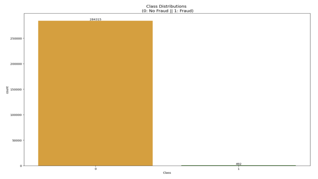
Imbalanced data set: Imbalanced classification involves developing predictive models on classification datasets that have severe class imbalances. The challenge of working with imbalanced datasets is that most machine learning techniques will ignore, and in turn have poor performance on, the minority class, although typically it is performance on the minority class that is most important. There are many examples of imbalanced datasets such as device failure rates, customer churns for a successful company, cancer prediction, etc.
Data Exploration
Let’s visualize the data and distribution of various features. We will use SelectKBestScores to rate the features, help us understand which features have heavy influence on which transactions are fraud, and help us understand correlation of the various parameters to “Fraud” or “No Fraud.”
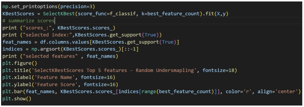
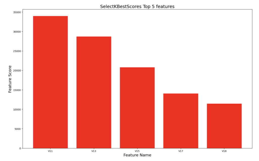
We can see that features v11, v13, v15, v17, and v18 are the top five features contributing to the “Fraud” transactions. Other techniques such as a correlation matrix will yield similar results.
Once we identify the top features, we can drill down on each feature and identify extreme outliers. We use a technique called interquartile range to identify extreme outliers that fall outside the range set by interquartile range.
Mitigating Class Imbalance
Random undersampling can be used to make the data more balanced by picking all the “No Fraud” cases (492 transactions) and concatenating with an equal number (492) of randomly picked “Fraud” cases to create a new sub-sample. Now the two classes have equal distribution. The caveat of this technique is that it suffers from the problem of information loss due to picking only 492 out of 284,315 “No Fraud” transactions, which isn’t ideal in terms of accuracy.
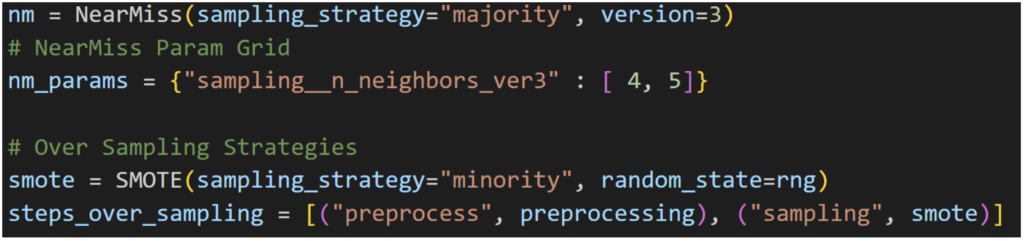
Note that there’s another undersampling technique called NearMiss that has a few variations. NearMiss-3 involves selecting a given number of majority class examples for each closest minority class example.
Another approach to addressing imbalanced datasets is to oversample the minority class. The simplest approach involves duplicating examples in the minority class, although these examples don’t add any new information to the model. Instead, new examples can be synthesized from the existing examples. This is a type of data augmentation for the minority class and is referred to as the Synthetic Minority Oversampling Technique, or SMOTE for short. Imbalanced-learn (imblearn), which is already part of Anaconda Distribution and specifically designed to work with imbalanced datasets. In particular, imbalanced-learn offers methods for data augmentation of test datasets. For an imbalanced dataset, accuracy doesn’t matter as much since the large majority of data falls in one class. What matters is the F1-score, since it takes both precision and recall into account.
The SMOTE technique has some disadvantages, especially for data with high dimensionality. When there is high dimensionality it can increase noise, impact variance, and increase correlation. But in our case, since the number of features in the dataset is small (around 30), it works well.
Depending on the dataset you can apply many more data preparation techniques, such as dimensionality reduction, etc.; we have focused on only a few commonly used techniques, but you should be able to apply others on AWS-Graviton-based instances with Anaconda Distribution without any issues.
The complete code used for this blog can be found here.
Train and Tune
After data preparation, the data is ready to be used for training and tuning.
For the above-mentioned dataset, we will primarily use an ML scikit-learn framework with decision tree and random forest classifiers for reasons covered below. There are other classifiers such as LogisticRegression, KNN, etc. that you can try, but we will focus on decision tree and random forest. It’s good to try out different classifiers to see which one works best with your dataset. DecisionTree is a classical ML algorithm and works well on CPUs.
Decision trees are widely used algorithms for supervised machine learning. They are popular for their ease of interpretation and large range of applications in banking (fraud detection, loan approval, etc.), healthcare, e-commerce, and more. They work for both regression and classification problems.
Decision trees have greater interpretability, which is important when the decision process may need to be explained to customers or for compliance reasons. CPUs are great for running decision trees, especially when the datasets are small. CPUs can be used for training as well as inferencing given that they are simpler to use in nature and generally cost less than GPUs.
We use GridSeacrhCV to tune the hyperparameters for DecisionTree() and RandomForest().
The following code shows how to instantiate the evaluation pipeline using the SMOTE oversampling strategy. Similarly, the pipeline could be created using NearMiss.
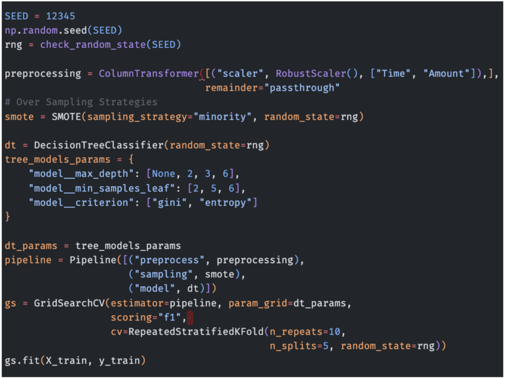
After creating the above pipeline, we train it and do predictions on held-out test data.
Metrics
As discussed earlier, for an imbalanced dataset, accuracy doesn’t much matter since the large majority of data falls in one class. What matters is the F1-score (higher is better), since it takes both precision and recall into account as well as the area under the ROC curve (AUC). So let’s look at these. We can see that the F1-score for SMOTE tends to outperform that of NearMiss:
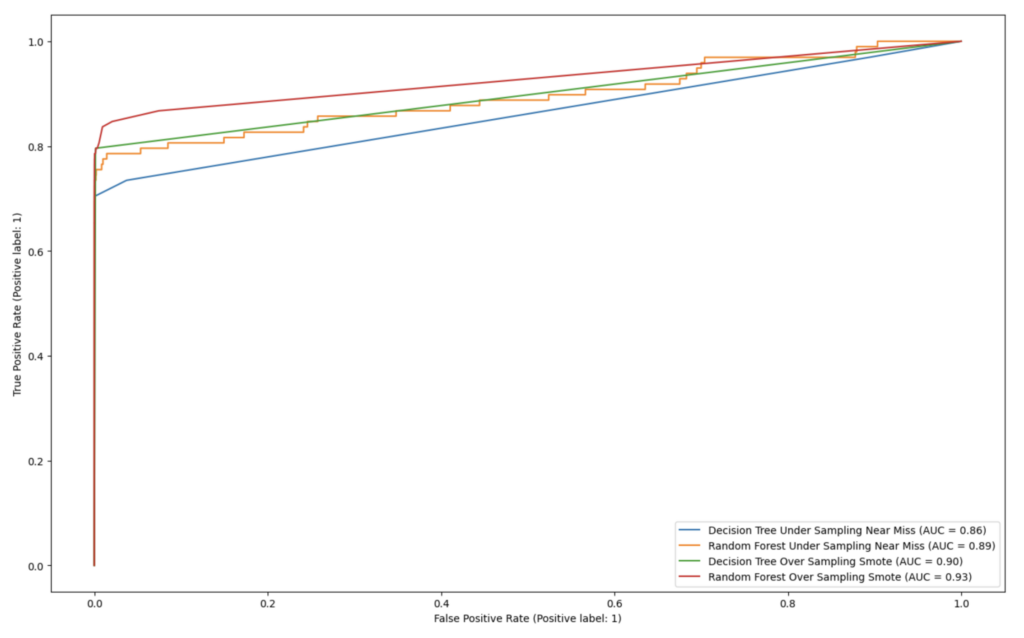
As we can see in the above chart, the SMOTE technique does indeed do a better job than the NearMiss technique, with both decision trees and random forest as classifiers. Also, RandomForest does slightly better than DecisonTree in terms of AUC.
| F1-score (higher is better) | DecisionTree (scikit-learn) Classifier | RandomForest (scikit-learn) Classifier |
| NearMiss undersampling technique | 0.75 | 0.77 |
| SMOTE technique | 0.61 | 0.82 |
Interpretability – Visualization of the Decision Tree
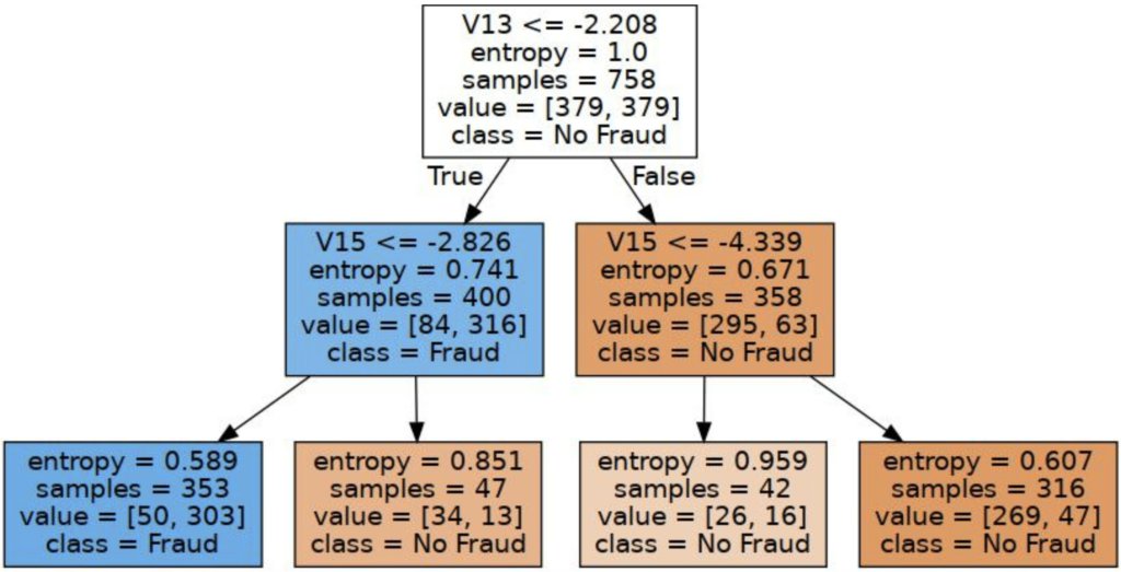
Below is a sub-section of the decision tree generated by the graphviz package (available through Anaconda Distribution), which shows the process of how the decision tree makes decisions based on inputs for the credit card fraud dataset.
In the code below, we leverage the export_graphviz utility function provided by scikit-learn to plot tree models in Graphviz Dot format. You would need to install both graphviz and python-graphviz to run this code, and both are available through conda install in Anaconda Distribution:
conda install graphviz python-graphviz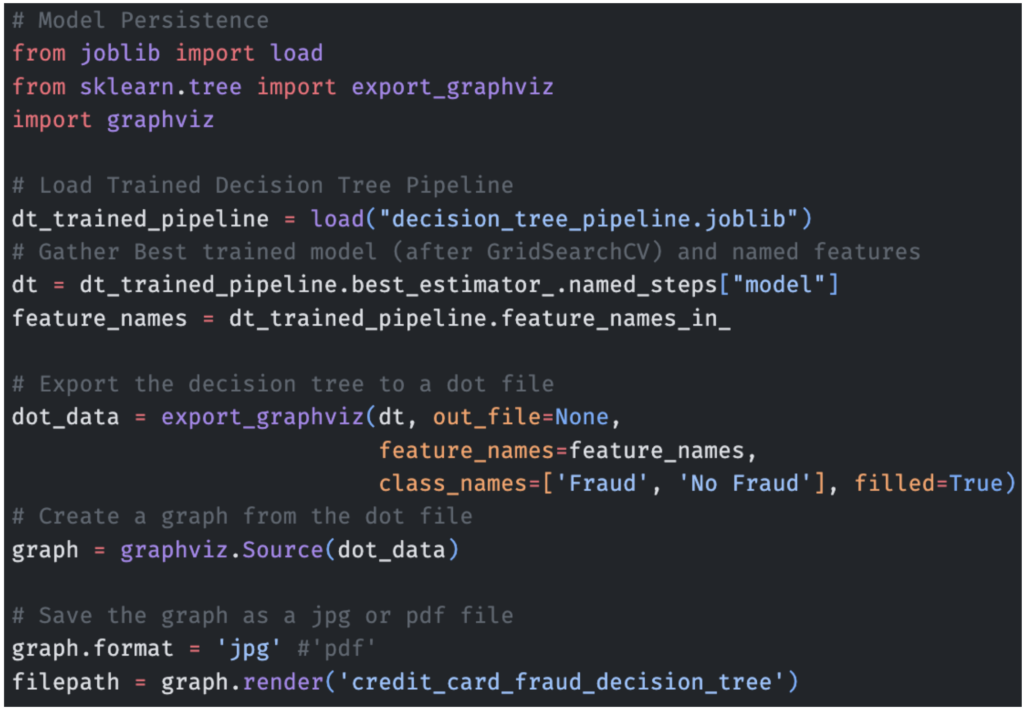
In the graphic below, we can see that if feature v13 has a value less than or equal to -2.208, the path goes to feature v15, which in turn looks at the threshold value of -2.826, and so on until we reach a leaf node. This is how we know deterministically how a transaction was classified as “Fraud” or “No Fraud.”
Deploy and Monitor
For deployment, Anaconda provides several packages that will be useful. ML containers are frequently used for deploying ML models. Anaconda Distribution supports Docker, conda-pack, mamba, etc. One can build multi-architecture ML packages for deploying to x86 and AWS-Graviton-based instances. The migration (or new deployment) of your models from x86-powered instances to Graviton instances is simple, because AWS provides containers to host models with PyTorch, TensorFlow, scikit-learn, and XGBoost, and the models are architecture agnostic. You can learn more about building multi-architecture containers here.
Anaconda assists in monitoring and maintaining deployed ML models. There are libraries that can be used for monitoring model performance, tracking data drift, and retraining models as necessary. Additionally, Anaconda provides version control integration, and Anaconda’s package management updates and bug fixes for ML libraries can easily be installed to ensure models stay up to date.
In the ML lifecycle, model training, testing, deployment, and inference are ongoing activities. It’s a good practice to continuously monitor these with metrics.
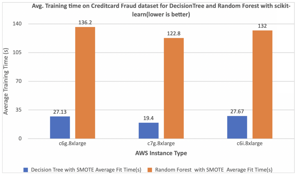
Model Training Time metric
The chart below shows a comparison of the training times on Graviton-based instances and x86-based instances for our models. For comparison, we used 3 different AWS instance types:
- c7g.8xlarge (AWS Graviton3)
- c6g.8xlarge (AWS Graviton2)
- c6i.8xlarge (3rd-generation Intel Xeon Scalable processors)
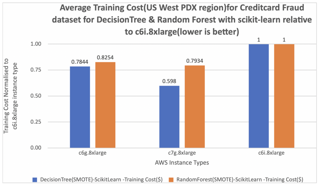
In the following graph, we measure the cost of training. We further normalize the cost per training results to a c6i.8xlarge instance, which is measured as 1 on the Y-axis of the chart. You can see that the cost per training for c7g.8xlarge (AWS Graviton3) is about 20% of that of the c6i.8xlarge for both DecisionTree and RandomForest classifiers using the scikit-learn framework.
As you can see in the chart below, the AWS-Graviton3-based instances (c7g.8xlarge) outperform the x86-based Amazon EC2 instance (c6i.8xlarge).
There are more details on the price and performance benefits (inference latency) of using AWS Graviton for inferencing for a wide variety of ML frameworks here.
Conclusion
Anaconda Distribution supports all major Python packages for arm64 that can run on AWS Graviton to ultimately complete a self-managed ML lifecycle on AWS Graviton. In this blog post, we considered a real-world use case of credit card fraud detection, and how AWS Graviton can be used to implement a full ML lifecycle. We demonstrated that the functionality generally available on x86-based AWS EC2 instances is also available on AWS Graviton to run ML workloads. Anaconda Distribution enabled this process to guarantee complete portability of the Python ML stack across different architectures. In the post, we also analyzed the performance of AWS Graviton, which offers ease of use in terms of debuggability as well as interpretability, as we saw for DecisionTree, which is desired for some ML workloads due to compliance and other requirements. AWS Graviton can be used for doing training and inferencing of some common classical ML workloads. AWS Graviton provides price and price-performance advantages and is supported by most AI/ML frameworks.
Resources and Further Reading
- Link to the code used in this blog: anaconda/ml-on-aws-graviton: Code and Replication Material attached to the “Implementing a full ML-lifecycle with Anaconda Distribution on AWS Graviton” Blog Post (github.com)
- AWS Graviton Fast Start Program: https://aws.amazon.com/ec2/graviton/fast-start/
- Amazon EC2 Graviton Burstable Instances:
- AWS Graviton Technical Guide:
- Optimized PyTorch 2.0 inference with AWS Graviton processors | AWS Machine Learning Blog (Amazon.com): https://aws.amazon.com/blogs/machine-learning/optimized-pytorch-2-0-inference-with-aws-graviton-processors/
- Run machine learning inference workloads on AWS-Graviton-based instances with Amazon SageMaker | AWS Machine Learning Blog: https://aws.amazon.com/blogs/machine-learning/run-machine-learning-inference-workloads-on-aws-graviton-based-instances-with-amazon-sagemaker/
- Reduce Amazon SageMaker inference cost with AWS Graviton | AWS Machine Learning Blog: https://aws.amazon.com/blogs/machine-learning/reduce-amazon-sagemaker-inference-cost-with-aws-graviton/
- ML Lifecycle using SageMaker: https://aws.amazon.com/blogs/machine-learning/architect-and-build-the-full-machine-learning-lifecycle-with-amazon-sagemaker/
- Interpretability versus explainability: https://docs.aws.amazon.com/whitepapers/latest/model-explainability-aws-ai-ml/interpretability-versus-explainability.html
- Anaconda | Announcing Anaconda Support on AWS Graviton2: https://anaconda.cloud/install-arm64-on-aws-graviton2
- Using AWS EC2 Graviton2-based instances with Anaconda: